Unlocking The Secrets of Algo Trading: Learn How to Use Python for Getting Data and Strategies…!!

With Python's limitless libraries and tools, we can build a robust foundation to predict market trends, analyse financial data, and create advanced financial models.

Hey there! In this post, I'm going to talk about setting things up for algo trading. [In my previous video], I covered many aspects of algo trading, including technology, tools, markets, and data. I will build on top of that in this blog post. I would like to point out that this post is accompanied by a video which I shared before.

You can watch the supplementary video and [Follow Along the Video].

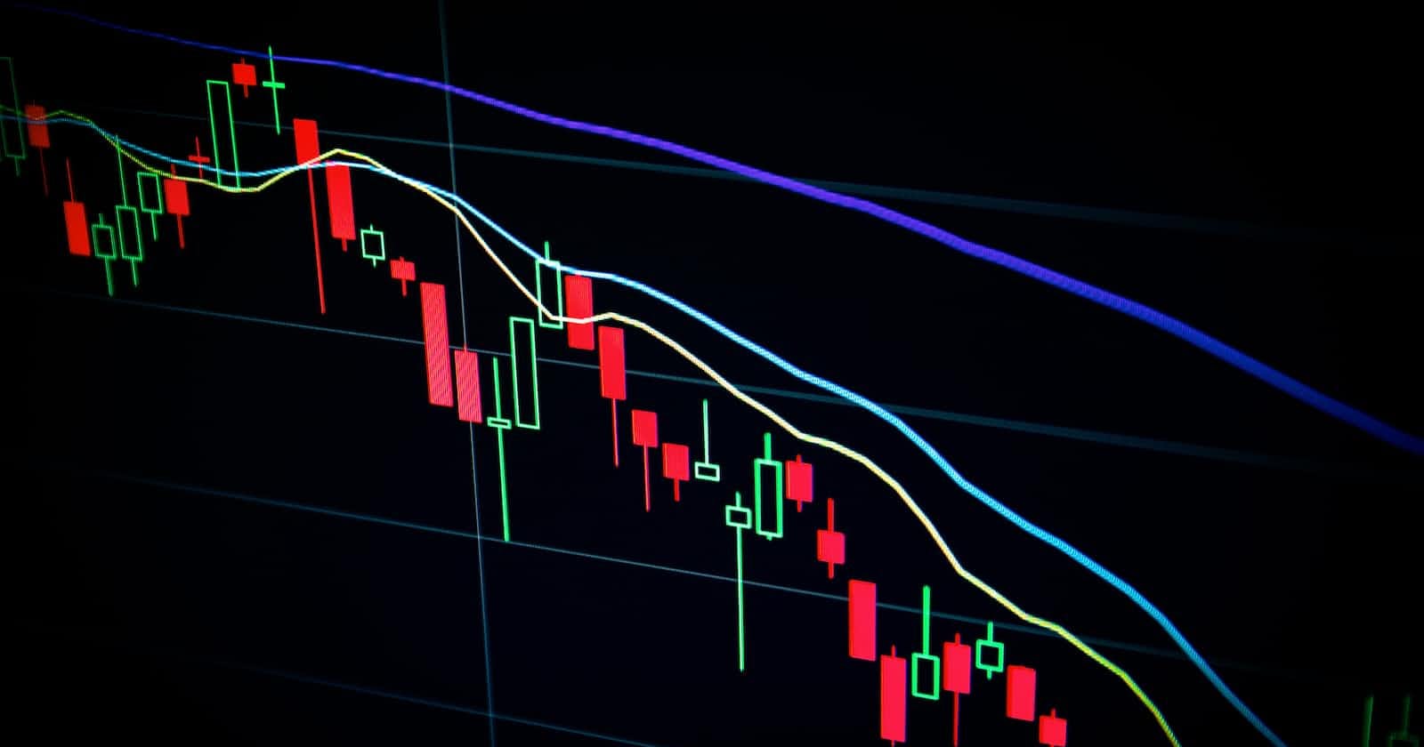
Hardware & Software Setup

You don't need a fancy computer for this, anything online or a simple computer will work.

8 GB of RAM with an i5 Processor. Something lower might work too.
Apple Silicon (m1/m2) is great too if you can install the required dependencies. There are few libraries which do not work on it.
Anaconda Environment with Python 3.7. Though higher version of python can be taken, however I have found this to be the common denominator which most libraries support.
List of Libraries to Install
- Pandas
- Numpy
- Matplotlib, Seaborn, Plotly
- yfinance
- Cufflinks
Bonus : Just use Google Colab and install yfinance, Cufflinks in there and get started

Here’s what we will focus on

We will be setting up a python environment, getting market data using Yahoo Finance, and doing some basic statistical analysis. We will then create a simple strategy and compare returns.

Get market data from Yahoo Finance.
Play with the data, get data from NSE, and do stats on it.
Calculate moving averages and do plotting.
Try to do something known as Bollinger bands, which is a technical indicator.
Make a simple moving average-based strategy.

More Details

After installing the libraries, we will use Yahoo Finance to get market data. We will define a variable ticker and set start and end dates. Then, we will download the data and create a data frame. We will also reduce the number of days to make it easier to plot.

Next, we will plot the high, lows, and search for patterns. We will also calculate some basic formulas like simple moving average, exponential moving averages, and Bollinger bands. Bollinger bands is a plus-minus two standard deviations up and down from a simple moving average.

Finally, we will make a simple moving average-based strategy. The strategy will be to sell if a condition is met and hold if it is not.

The Complete Code is shared below

Install necessary libraries.
Define variable ticker and set start and end dates.
Download data and create a data frame.
Reduce the number of days to make it easier to plot.
Plot high lows and search for patterns.
Calculate basic formulas like simple moving average, exponential moving averages, and Bollinger bands.

Working with a Strategy

In the world of algorithmic trading, having a well-defined strategy is crucial for success. A trading strategy is simply a set of rules that traders follow to generate signals that indicate when to buy, sell, or do nothing.

One popular trading strategy is using the simple moving average (SMA). The SMA is a technical indicator that helps traders identify trends in the market. It calculates the average price of a security over a specific time period, such as 12 days, by adding up the closing prices of each day and dividing it by the number of days in the period.

When using the SMA, traders typically buy a stock when its closing price is higher than its simple moving average and sell it when the closing price is lower. This approach can help traders identify potential uptrends or downtrends in the market and make informed decisions on when to enter or exit a trade.

However, it's important to note that no trading strategy is foolproof. Market conditions can change rapidly, and unforeseen events can impact a stock's performance. Therefore, it's essential to continually monitor the market and adjust trading strategies as needed.

In addition to the SMA, there are many other technical indicators and trading strategies that traders can use to make informed decisions in the market. Some popular ones include the relative strength index (RSI), the moving average convergence divergence (MACD), and the Bollinger Bands.

When studying financial engineering and data science, it's essential to clean up data to ensure that the calculations are accurate. This often involves dropping unnecessary columns and removing any errors or outliers that may skew the results.

In summary, having a well-defined trading strategy is essential for success in algorithmic trading. The SMA is just one of many technical indicators and trading strategies that traders can use to make informed decisions in the market. However, it's important to continually monitor the market and adjust strategies as needed to stay ahead of the game.

Complete Code

#pip install yfinance plotly cufflinks

# Core Imports
import pandas as pd
import numpy as np
import datetime
import yfinance as yf
import matplotlib.pyplot as plt

#Ticker is the stock that we want to get
Ticker = "^NSEI"


# Get Sample data based on a Ticker
end1 = datetime.date.today()
start1 = end1 - pd.Timedelta(days=5)

df = yf.download(Ticker, start=start1, end=end1, interval="5m" )
print(df.head())
df.info()

# Plotting the Data

df1a = df.copy()
df1a.loc['2023-02-13', ['Open', 'High', 'Low', 'Close']].plot(grid=True, linewidth=1, figsize=(14, 9))

# Just the Closing Price
df1a['Close'].plot(grid=True, linewidth=1, figsize=(14, 9))

# Core Calculation Functions 
# SMA
def get_sma(prices, rate):
  return prices.rolling(rate).mean()

# EMA
def get_ema(prices, rate):
  return prices.ewm(span=ema, adjust=False).mean()

# Bollinger Bands

# Bollinger bands are a technical analysis tool used by traders to identify potential entry and exit points in the market. They are created by plotting a moving average of the price along with two standard deviation lines above and below it. By doing so, Bollinger bands can provide an indication of whether a stock is overbought or oversold. They also help traders identify potential breakouts or reversals in the market. With this knowledge, traders can make more informed decisions when entering or exiting a position in the market.

def get_bollinger_bands(prices,rate):
    sma = get_sma(prices, rate)
    std = prices.rolling(rate).std()
    bollinger_up = sma + std * 2 # Calculate top band
    bollinger_down = sma - std * 2 # Calculate bottom band
    return bollinger_up, bollinger_down


# Other Functions

def download_daily_data(ticker, start, end):
    """ 
    The function downloads daily market data to a pandas DataFrame 
    using the 'yfinance' API between the dates specified.
    """
    data = yf.download(ticker, start, end)

    return data

def compute_daily_returns(data):
    """ 
    The function computes daily log returns based on the Close prices in the pandas DataFrame
    and stores it in a column  called 'cc_returns'.
    """
    data['cc_returns'] = np.log(data['Close'] / data['Close'].shift(1))
    return data

# Generate Bollinger bands for the above

bollinger_up, bollinger_down = get_bollinger_bands(df1a['Close'],20)


# Plot the Results

symbol = 'NSE'
closing_prices = df1a['Close']

plt.title(symbol + ' Bollinger Bands')
plt.xlabel('Days')
plt.ylabel('Closing Prices')
plt.plot(closing_prices, label='Closing Prices')
plt.plot(bollinger_up, label='Bollinger Up', c='g')
plt.plot(bollinger_down, label='Bollinger Down', c='r')
plt.legend()
plt.show()


# Strategy Perform Calculations

# Remove the Un-necessary Columns
df1a.drop(columns=['High', 'Low', 'Volume'], inplace=True)

# Create a new colum which captures the percentage cahnge from previous day
df1a['cc_returns'] = df1a['Close'].pct_change()

# Define a short 12 day sma 
sma = 12
df1a['sma'] = df1a['Close'].rolling(window=sma).mean()

print(df1a.head())
print(df1a.tail())

# If the closging price is higher that sma buy else do nothing
df1a['position'] = np.where((df1a['Close'] > df1a['sma']), 1, 0)
df1a['position'] = df1a['position'].shift(1)
df1a['position'].value_counts()

# Plotting the above strategy returns

df1a['strategy_returns'] = df1a['cc_returns'] * df1a['position']


df1a['strategy_returns'] = 1 + df1a['strategy_returns']
df1a['cc_returns'] = 1 + df1a['cc_returns']

print(df1a.head())
print(df1a.tail())

df1a[['cc_returns', 'strategy_returns']].cumprod().plot(grid=True, figsize=(9, 5))

print('Buy and hold returns: ', np.round(df1a['cc_returns'].cumprod()[-1], 2))
print('Strategy returns: ', np.round(df1a['strategy_returns'].cumprod()[-1], 2))
HyperWrite Logo